The Dataset

To train this mammoth of a model, a mammoth of a dataset is also needed. The datasets from all three submodels - MiDAS, YoloV3 and PlaneRCNN - had to be combined.

The first thought was to make use of pytorch’s ConcatDataset, but this was quickly discarded since it does not sync the three datasets.

MiDAS Dataset

The MiDAS dataset had to contain the depth maps of all the input images. Inference was run using the original MiDAS repo and the generated depth maps were used as ground truths. Nothing too hard here.

YoloV3 Dataset

Using the knowledge gained during assignment 13, making use of the LoadImagesAndLabels dataset class from the YoloV3 repo took no effort (kinda). The code was slightly modified though, to return the letterbox padding extents as well, which will be used in the loss function later on. Also, any augmentations that the class did was turned off.

PlaneRCNN Dataset

This is where things got really messy. PlaneRCNN was trained on ScanNet, and the custom dataset that we are training on is completely different from ScanNet. The dataset classes in the PlaneRCNN repo made a lot of references to ScanNet in their code. So instead of tackling the dataset, the model was looked at.

The model took quite a number of arguments during inference, being image_metas, gt_class_ids, gt_boxes, gt_masks, gt_parameters and camera. Moreover, the calculation of the loss depended on even more parameters, being rpn_match, rpn_bbox, rpn_class_logits, rpn_pred_bbox, target_class_ids, mrcnn_class_logits, target_deltas, mrcnn_bbox, target_mask, mrcnn_mask, target_parameters and mrcnn_parameters. So the source of all these parameters had to be found out.

As luck would have had it, the sources of all those gazillion parameters were just three things, the input image, the segmentation / mask and the parameters. Now the sources of the segmentation / mask and the parameters had to be figured out. It turns out that the parameters are given during inference of the original PlaneRCNN, however, the segmentation / mask was not that simple to obtain from the inferences generated from the original PlaneRCNN model.

The PlaneRCNN repo gave a hint on how the segmentation map should be like:

“…In our implementation, we use one 2D segmentation map where pixels with value i belong to the ith plane in the list.”

This would mean that if PlaneRCNN detects 15 planes, there would be 15 masks, and the 2D segmentation map should be constructed in such a way that the 0th plane should have all 0’s as its mask value in the segmentation map, the 1st plane should have all 1’s as its mask value in the segmentation map and so on.

Diving into the PlaneRCNN code a bit more, the generated masks during inference contain the mask information as mentioned above, and this array was saved as an .npy file during inference. Now another problem cropped up. Each of these .npy files were around an average of 20mb, which would mean that the PlaneRCNN dataset would be around 20 * 3000 = 60000 mb = 60gb!

The huge size of each faile was due to the fact that if the PlaneRCNN model detected 15 planes, the array stored in the .npy file would have a shape of (P, H, W) where P is the number of planes (here 15), H is the height of the image, and W is the width. This discovery further soldified the hypothesis that was made after reading the hint in the PlaneRCNN repo. Now the question was how to reduce this file size. Surprisingly, the answer came from an unexpected source: ScanNet.

ScanNet’s segmentation maps were an RGB image in which each plane was denoted with a color. So converting the (P, H, W) array into an RGB image would save a huge amount of space. After a bit of research into representations of RGB images as integers, the following three functions were used to convert to and fro between the .npy file and the segmentation RGB image.

def masks_to_image(masks):
    # shape of masks should be (H, W, N)
    # toRGB = lambda x: (x // 256 // 256 % 256, x // 256 % 256, x % 256)
    toRGB = lambda x: (x >> 16 & 255, x >> 8 & 255, x & 255)
    max_val = 16777215

    step = max_val // (masks.shape[2])
    img = np.full((masks.shape[0], masks.shape[1], 3), fill_value=0, dtype=np.int32)

    for i in range(1, masks.shape[2] + 1):
        img[masks[:, :, i - 1] == 1] = toRGB(i * step)

    return img # (H, W, C)

def image_to_mask(img, num_masks):
    # img shape should be (H, W, C) and type should be int
    img = img.astype(np.int32)

    max_val = 16777215
    step = max_val // num_masks
    return ((img[:, :, 0] * 256 * 256 + img[:, :, 1] * 256 + img[:, :, 2]) // step) - 1

def image_to_masks(img, num_masks):
    # img shape should be (H, W, C) and type should be int
    img = img.astype(np.int32)

    m = image_to_mask(img, num_masks)
    masks = np.full((num_masks, m.shape[0], m.shape[1]), fill_value=0, dtype=np.int32)

    for i in range(num_masks):
        masks[i, m == i] = 1

    return masks # (N, H, W)

the function masks_to_image converted the .npy file contents to a RGB segmentation image, image_to_mask converted the RGB segmentation image to the format specified in the hint, and the image_to_masks function converted the RGB segmentation image back into the .npy file contents.The PlaneRCNN inference code was changed to use these functions instead. This lead to a huge decrease in the file size, from ~20mb to a couple of kilobytes. This notebook was used to generate the dataset for planercnn.

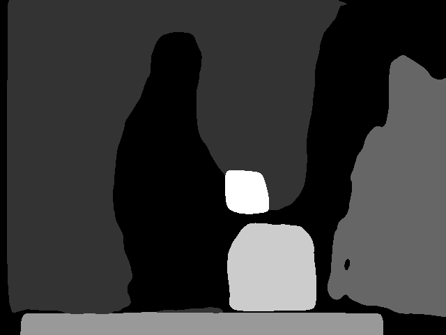
Example of a segmentation image generated by PlaneRCNN and the above code.

Now since that was was dealt with, the PlaneRCNN dataset code (specifically, the PlaneDatasetSingle class), was read through and the ScanNet related code was removed. Once done, the dataset was tested and it worked.